

Related Posts


Conversation Starter


Chief
Incoming multi-tier cringe




Coach
Additional Posts in Excel Genius

Coach



Visual Storyteller
New to Fishbowl?
Download the Fishbowl app to
unlock all discussions on Fishbowl.
unlock all discussions on Fishbowl.


Deeply resent being referred to so colloquially as an “Excel head” and will be reporting you to my Human Resources Generalist.
Oh, wait…
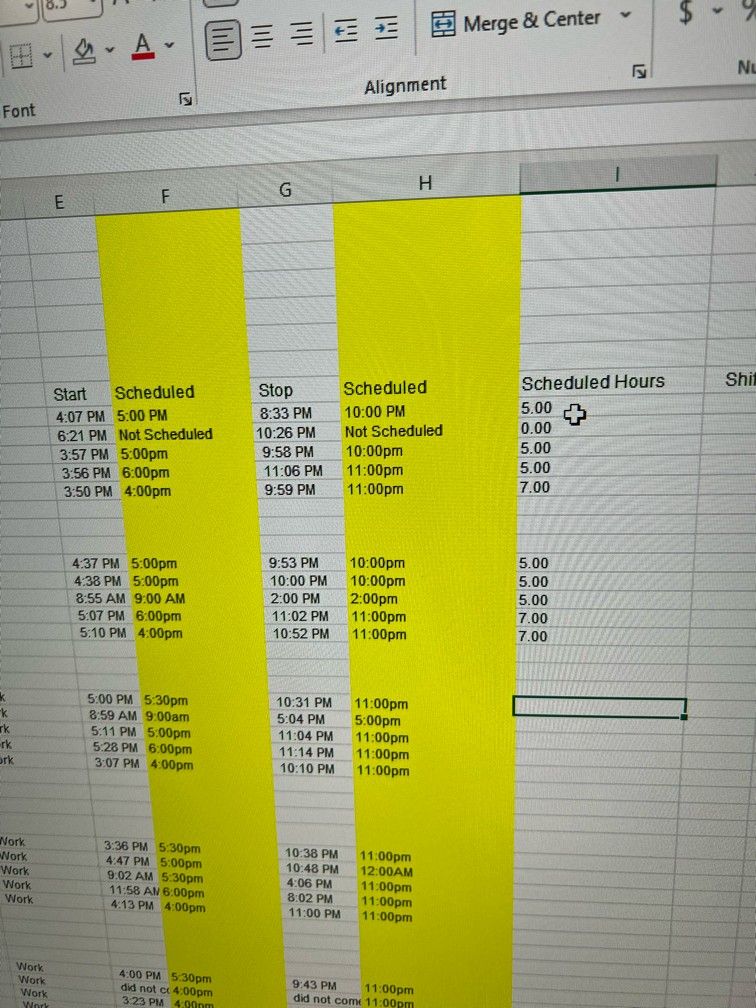
Show your formula so we can advise on what's wrong. The amounts in column I appear to be the correct expected value so not sure where you may be going wrong.
Because you say you're using a SUM formula, why wouldn't you take the value in column H less the value in column F?
Yeah, to get total time elapsed, I’d subtract column H from F. The difference should be 5 as displayed in column I… you can do the same thing for column G and E. But I would definitely make sure that all columns are time formatted… or number formatted if you just want the number
Add two helper columns and Convert time in both columns (H&F) to minutes and then add Both Helper columns. Then convert Minutes into 24 Hour format
Only numbers can do math, check the columns using =ISNUMBER(F1) and verify they are numbers. If not, use =NUMBERVALUE(F1) to get it to a number.
I think you meant to do H - F.
Make sure all columns you’re using are the same format.
SUM(date_time...) yields a time_value as DAYS
(stop-start) does the same. Just FORMAT as hours and minutes without "pm", to make sense of it.
24*SUM(date_time) yields hours
you can use =(F15-H15)*24-9